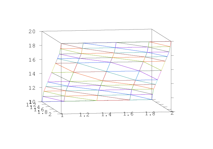
Figure 22.6: Example finite element model the showing triangular elements. The height of each vertex corresponds to the solution value.
Previous: Iterative Techniques, Up: Sparse Matrices [Contents][Index]
A common application for sparse matrices is in the solution of Finite Element Models. Finite element models allow numerical solution of partial differential equations that do not have closed form solutions, typically because of the complex shape of the domain.
In order to motivate this application, we consider the boundary value Laplace equation. This system can model scalar potential fields, such as heat or electrical potential. Given a medium Omega with boundary dOmega. At all points on the dOmega the boundary conditions are known, and we wish to calculate the potential in Omega. Boundary conditions may specify the potential (Dirichlet boundary condition), its normal derivative across the boundary (Neumann boundary condition), or a weighted sum of the potential and its derivative (Cauchy boundary condition).
In a thermal model, we want to calculate the temperature in Omega and know the boundary temperature (Dirichlet condition) or heat flux (from which we can calculate the Neumann condition by dividing by the thermal conductivity at the boundary). Similarly, in an electrical model, we want to calculate the voltage in Omega and know the boundary voltage (Dirichlet) or current (Neumann condition after diving by the electrical conductivity). In an electrical model, it is common for much of the boundary to be electrically isolated; this is a Neumann boundary condition with the current equal to zero.
The simplest finite element models will divide
Omega
into simplexes (triangles in 2D, pyramids in 3D).
We take as a 3-D example a cylindrical liquid filled tank with a small
non-conductive ball from the EIDORS project11. This is model is designed to reflect
an application of electrical impedance tomography, where current patterns
are applied to such a tank in order to image the internal conductivity
distribution. In order to describe the FEM geometry, we have a matrix of
vertices nodes and simplices elems.
The following example creates a simple rectangular 2-D electrically conductive medium with 10 V and 20 V imposed on opposite sides (Dirichlet boundary conditions). All other edges are electrically isolated.
   node_y = [1;1.2;1.5;1.8;2]*ones(1,11);
   node_x = ones(5,1)*[1,1.05,1.1,1.2, ...
             1.3,1.5,1.7,1.8,1.9,1.95,2];
   nodes = [node_x(:), node_y(:)];

   [h,w] = size (node_x);
   elems = [];
   for idx = 1:w-1
     widx = (idx-1)*h;
     elems = [elems; ...
       widx+[(1:h-1);(2:h);h+(1:h-1)]'; ...
       widx+[(2:h);h+(2:h);h+(1:h-1)]' ];
   endfor

   E = size (elems,1); # No. of simplices
   N = size (nodes,1); # No. of vertices
   D = size (elems,2); # dimensions+1
This creates a N-by-2 matrix nodes and a E-by-3 matrix
elems with values, which define finite element triangles:
  nodes(1:7,:)'
    1.00 1.00 1.00 1.00 1.00 1.05 1.05 …
    1.00 1.20 1.50 1.80 2.00 1.00 1.20 …

  elems(1:7,:)'
    1    2    3    4    2    3    4 …
    2    3    4    5    7    8    9 …
    6    7    8    9    6    7    8 …
Using a first order FEM, we approximate the electrical conductivity
distribution in
Omega
as constant on each simplex (represented by the vector conductivity).
Based on the finite element geometry, we first calculate a system (or
stiffness) matrix for each simplex (represented as 3-by-3 elements on the
diagonal of the element-wise system matrix SE). Based on SE
and a N-by-DE connectivity matrix C, representing the connections
between simplices and vertices, the global connectivity matrix S is
calculated.
  ## Element conductivity
  conductivity = [1*ones(1,16), ...
         2*ones(1,48), 1*ones(1,16)];

  ## Connectivity matrix
  C = sparse ((1:D*E), reshape (elems', ...
         D*E, 1), 1, D*E, N);

  ## Calculate system matrix
  Siidx = floor ([0:D*E-1]'/D) * D * ...
         ones(1,D) + ones(D*E,1)*(1:D) ;
  Sjidx = [1:D*E]'*ones (1,D);
  Sdata = zeros (D*E,D);
  dfact = factorial (D-1);
  for j = 1:E
     a = inv ([ones(D,1), ...
         nodes(elems(j,:), :)]);
     const = conductivity(j) * 2 / ...
         dfact / abs (det (a));
     Sdata(D*(j-1)+(1:D),:) = const * ...
         a(2:D,:)' * a(2:D,:);
  endfor
  ## Element-wise system matrix
  SE = sparse(Siidx,Sjidx,Sdata);
  ## Global system matrix
  S = C'* SE *C;
The system matrix acts like the conductivity
S
in Ohm’s law
S * V = I.
Based on the Dirichlet and Neumann boundary conditions, we are able to
solve for the voltages at each vertex V.
  ## Dirichlet boundary conditions
  D_nodes = [1:5, 51:55];
  D_value = [10*ones(1,5), 20*ones(1,5)];

  V = zeros (N,1);
  V(D_nodes) = D_value;
  idx = 1:N; # vertices without Dirichlet
             # boundary condns
  idx(D_nodes) = [];

  ## Neumann boundary conditions.  Note that
  ## N_value must be normalized by the
  ## boundary length and element conductivity
  N_nodes = [];
  N_value = [];

  Q = zeros (N,1);
  Q(N_nodes) = N_value;

  V(idx) = S(idx,idx) \ ( Q(idx) - ...
            S(idx,D_nodes) * V(D_nodes));
Finally, in order to display the solution, we show each solved voltage value in the z-axis for each simplex vertex. See Figure 22.6.
  elemx = elems(:,[1,2,3,1])';
  xelems = reshape (nodes(elemx, 1), 4, E);
  yelems = reshape (nodes(elemx, 2), 4, E);
  velems = reshape (V(elemx), 4, E);
  plot3 (xelems,yelems,velems,"k");
  print "grid.eps";

Figure 22.6: Example finite element model the showing triangular elements. The height of each vertex corresponds to the solution value.
EIDORS - Electrical Impedance Tomography and Diffuse optical Tomography Reconstruction Software http://eidors3d.sourceforge.net
Previous: Iterative Techniques, Up: Sparse Matrices [Contents][Index]