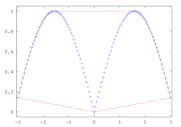
Figure 30.5: The convex hull of a simple set of points
Next: Interpolation on Scattered Data, Previous: Voronoi Diagrams, Up: Geometry [Contents][Index]
The convex hull of a set of points is the minimum convex envelope
containing all of the points. Octave has the functions convhull
and convhulln to calculate the convex hull of 2-dimensional and
N-dimensional sets of points.
Compute the convex hull of the set of points defined by the arrays x and y. The hull H is an index vector into the set of points and specifies which points form the enclosing hull.
An optional third argument, which must be a string or cell array of strings,
contains options passed to the underlying qhull command.
See the documentation for the Qhull library for details
http://www.qhull.org/html/qh-quick.htm#options.
The default option is {"Qt"}.
If options is not present or [] then the default arguments are
used. Otherwise, options replaces the default argument list.
To append user options to the defaults it is necessary to repeat the
default arguments in options. Use a null string to pass no arguments.
Compute the convex hull of the set of points pts.
pts is a matrix of size [n, dim] containing n points in a space of dimension dim.
The hull h is an index vector into the set of points and specifies which points form the enclosing hull.
An optional second argument, which must be a string or cell array of strings, contains options passed to the underlying qhull command. See the documentation for the Qhull library for details http://www.qhull.org/html/qh-quick.htm#options. The default options depend on the dimension of the input:
{"Qt"}
{"Qt", "Qx"}
If options is not present or [] then the default arguments are
used. Otherwise, options replaces the default argument list.
To append user options to the defaults it is necessary to repeat the
default arguments in options. Use a null string to pass no arguments.
If the second output v is requested the volume of the enclosing convex hull is calculated.
An example of the use of convhull is
x = -3:0.05:3;
y = abs (sin (x));
k = convhull (x, y);
plot (x(k), y(k), "r-", x, y, "b+");
axis ([-3.05, 3.05, -0.05, 1.05]);
The output of the above can be seen in Figure 30.5.
Next: Interpolation on Scattered Data, Previous: Voronoi Diagrams, Up: Geometry [Contents][Index]