Next: Vector Rotation Matrices, Previous: Convex Hull, Up: Geometry [Contents][Index]
30.4 Interpolation on Scattered Data
An important use of the Delaunay tessellation is that it can be used to
interpolate from scattered data to an arbitrary set of points. To do
this the N-simplex of the known set of points is calculated with
delaunay or delaunayn. Then the simplices in to which the
desired points are found are identified. Finally the vertices of the simplices
are used to interpolate to the desired points. The functions that perform this
interpolation are griddata, griddata3 and griddatan.
- : zi = griddata (x, y, z, xi, yi) 
- : zi = griddata (x, y, z, xi, yi, method) 
- : [xi, yi, zi] = griddata (…) 
- : vi = griddata (x, y, z, v, xi, yi, zi) 
- : vi = griddata (x, y, z, v, xi, yi, zi, method) 
- : vi = griddata (x, y, z, v, xi, yi, zi, method, options) 
-
Interpolate irregular 2-D and 3-D source data at specified points.
For 2-D interpolation, the inputs x and y define the points where the function
z = f (x, y)is evaluated. The inputs x, y, z are either vectors of the same length, or the unequal vectors x, y are expanded to a 2-D grid withmeshgridand z is a 2-D matrix matching the resulting size of the X-Y grid.The interpolation points are (xi, yi). If, and only if, xi is a row vector and yi is a column vector, then
meshgridwill be used to create a mesh of interpolation points.For 3-D interpolation, the inputs x, y, and z define the points where the function
v = f (x, y, z)is evaluated. The inputs x, y, z are either vectors of the same length, or if they are of unequal length, then they are expanded to a 3-D grid withmeshgrid. The size of the input v must match the size of the original data, either as a vector or a matrix.The optional input interpolation method can be
"nearest","linear", or for 2-D data"v4". When the method is"nearest", the output vi will be the closest point in the original data (x, y, z) to the query point (xi, yi, zi). When the method is"linear", the output vi will be a linear interpolation between the two closest points in the original source data in each dimension. For 2-D cases only, the"v4"method is also available which implements a biharmonic spline interpolation. If method is omitted or empty, it defaults to"linear".For 3-D interpolation, the optional argument options is passed directly to Qhull when computing the Delaunay triangulation used for interpolation. For more information on the defaults and how to pass different values, see
delaunayn.Programming Notes: If the input is complex the real and imaginary parts are interpolated separately. Interpolation is normally based on a Delaunay triangulation. Any query values outside the convex hull of the input points will return
NaN. However, the"v4"method does not use the triangulation and will return values outside the original data (extrapolation).
- : vi = griddata3 (x, y, z, v, xi, yi, zi) 
- : vi = griddata3 (x, y, z, v, xi, yi, zi, method) 
- : vi = griddata3 (x, y, z, v, xi, yi, zi, method, options) 
-
Interpolate irregular 3-D source data at specified points.
The inputs x, y, and z define the points where the function
v = f (x, y, z)is evaluated. The inputs x, y, z are either vectors of the same length, or if they are of unequal length, then they are expanded to a 3-D grid withmeshgrid. The size of the input v must match the size of the original data, either as a vector or a matrix.The interpolation points are specified by xi, yi, zi.
The optional input interpolation method can be
"nearest"or"linear". When the method is"nearest", the output vi will be the closest point in the original data (x, y, z) to the query point (xi, yi, zi). When the method is"linear", the output vi will be a linear interpolation between the two closest points in the original source data in each dimension. If method is omitted or empty, it defaults to"linear".The optional argument options is passed directly to Qhull when computing the Delaunay triangulation used for interpolation. See
delaunaynfor information on the defaults and how to pass different values.Programming Notes: If the input is complex the real and imaginary parts are interpolated separately. Interpolation is based on a Delaunay triangulation and any query values outside the convex hull of the input points will return
NaN.
- : yi = griddatan (x, y, xi) 
- : yi = griddatan (x, y, xi, method) 
- : yi = griddatan (x, y, xi, method, options) 
-
Interpolate irregular source data x, y at points specified by xi.
The input x is an MxN matrix representing M points in an N-dimensional space. The input y is a single-valued column vector (Mx1) representing a function evaluated at the points x, i.e.,
y = fcn (x). The input xi is a list of points for which the function output yi should be approximated through interpolation. xi must have the same number of columns (N) as x so that the dimensionality matches.The optional input interpolation method can be
"nearest"or"linear". When the method is"nearest", the output yi will be the closest point in the original data x to the query point xi. When the method is"linear", the output yi will be a linear interpolation between the two closest points in the original source data. If method is omitted or empty, it defaults to"linear".The optional argument options is passed directly to Qhull when computing the Delaunay triangulation used for interpolation. See
delaunaynfor information on the defaults and how to pass different values.Example
## Evaluate sombrero() function at irregular data points
x = 16*gallery ("uniformdata", [200,1], 1) - 8;
y = 16*gallery ("uniformdata", [200,1], 11) - 8;
z = sin (sqrt (x.^2 + y.^2)) ./ sqrt (x.^2 + y.^2);
## Create a regular grid and interpolate data
[xi, yi] = ndgrid (linspace (-8, 8, 50));
zi = griddatan ([x, y], z, [xi(:), yi(:)]);
zi = reshape (zi, size (xi));
## Plot results
clf ();
plot3 (x, y, z, "or");
hold on
surf (xi, yi, zi);
legend ("Original Data", "Interpolated Data");
Programming Notes: If the input is complex the real and imaginary parts are interpolated separately. Interpolation is based on a Delaunay triangulation and any query values outside the convex hull of the input points will return
NaN. For 2-D and 3-D data additional interpolation methods are available by using thegriddatafunction.
An example of the use of the griddata function is
rand ("state", 1);
x = 2*rand (1000,1) - 1;
y = 2*rand (size (x)) - 1;
z = sin (2*(x.^2+y.^2));
[xx,yy] = meshgrid (linspace (-1,1,32));
zz = griddata (x, y, z, xx, yy);
mesh (xx, yy, zz);
that interpolates from a random scattering of points, to a uniform grid. The output of the above can be seen in Figure 30.6.
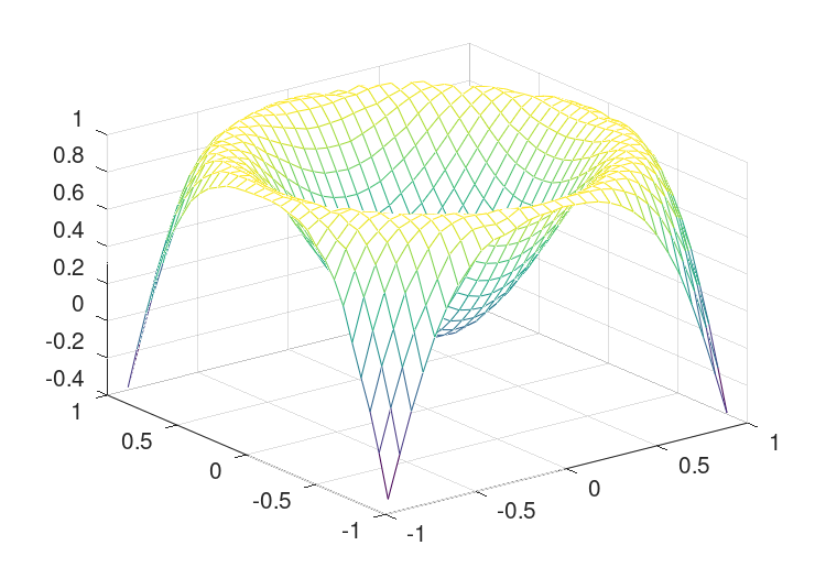
Figure 30.6: Interpolation from a scattered data to a regular grid